Motivation
This blog is the second one of my 3 blogs about VAR model. In this blog, I will introduce how to use Stata’s integrated commands var and svar to estimate the VAR model, which is also the common practices for researchers in VAR estimation. While it has little incremental value to an extant blog Vector autoregressions in Stata written by David Schenck, this blog will serve as an important benchmark for my manual calculations of all the major VAR estimation outputs in the next blog.
Sample Dataset
The dataset used in this blog is a shipped dataset named varsample.dta. It can be accessed here. This dataset collects the quarterly times series of U.S. unemployment rate unrate, rate of consumer price inflation inflation, and short-term nominal interest rate (federal funds rate) ffr from 1968 to 2018.
 1
 2
 3
 4
 5
 6
 7
 8
 9
10
11
12
|
. use varsample.dta, clear
. list in 1/5

     +---------------------------------------------------------+
     |     n_date         date    ffr   inflat~n   unrate   yq |
     |---------------------------------------------------------|
  1. | 1968-01-01   1968-01-01    4.5      -.659      3.7   32 |
  2. | 1968-04-01   1968-04-01    5.5      -.656      3.5   33 |
  3. | 1968-07-01   1968-07-01   6.13      -.651      3.7   34 |
  4. | 1968-10-01   1968-10-01      6      -.647      3.4   35 |
  5. | 1969-01-01   1969-01-01      4      -.643      3.4   36 |
     +---------------------------------------------------------+
|
Set time series (tsset or xtset)
The prerequisite for var and svar is a well-defined consecutive time series. As the sample data is not panel data, I use tsset to do that. The consecutive quarterly time series variable in this dataset is yq.
1
2
3
4
|
. tsset yq

Time variable: yq, 32 to 235
        Delta: 1 unit
|
Determine the time lag (varsoc)
I use varsoc command to run the lag-order selection. One can help varsoc to learn more details about the selection method. Both the likelihood ratio test and Akaike’s information criterion (AIC) recommend 7 lags, which I use through the rest of this post.
 1
 2
 3
 4
 5
 6
 7
 8
 9
10
11
12
13
14
15
16
17
18
19
20
21
|
. varsoc inflation unrate ffr, maxlag(8)

Lag-order selection criteria

   Sample: 40 thru 235                                     Number of obs = 196
  +---------------------------------------------------------------------------+
  | Lag |    LL      LR      df    p     FPE       AIC      HQIC      SBIC    |
  |-----+---------------------------------------------------------------------|
  |   0 | -1063.21                     10.6553   10.8797      10.9   10.9299  |
  |   1 |  170.566  2467.6    9  0.000  .00004  -1.61802  -1.53676  -1.41732  |
  |   2 |  217.394  93.657    9  0.000 .000027  -2.00402  -1.86183   -1.6528  |
  |   3 |  246.843  58.898    9  0.000 .000022  -2.21269  -2.00955* -1.71094* |
  |   4 |   253.46  13.233    9  0.152 .000023  -2.18837  -1.92429  -1.53609  |
  |   5 |   261.64  16.359    9  0.060 .000023     -2.18  -1.85498  -1.37719  |
  |   6 |  273.936  24.593    9  0.003 .000022  -2.21363  -1.82768   -1.2603  |
  |   7 |  285.311  22.751*   9  0.007 .000021* -2.23787* -1.79098  -1.13401  |
  |   8 |   289.68  8.7374    9  0.462 .000023  -2.19061  -1.68278  -.936231  |
  +---------------------------------------------------------------------------+
   * optimal lag
   Endogenous: inflation unrate ffr
    Exogenous: _cons
|
Estimate the VAR system (var or svar)
Having decided that the 7 lags are appropriate for this VAR, we can use either var or svar command to estimate the coefficients of the VAR. Theoretically we need to decide whether the VAR system is stable before the VAR estimation but we can usually skip this step because the VAR estimation would not converge if the system were not stable.
var command
The var command and results are as follows.
  1
  2
  3
  4
  5
  6
  7
  8
  9
 10
 11
 12
 13
 14
 15
 16
 17
 18
 19
 20
 21
 22
 23
 24
 25
 26
 27
 28
 29
 30
 31
 32
 33
 34
 35
 36
 37
 38
 39
 40
 41
 42
 43
 44
 45
 46
 47
 48
 49
 50
 51
 52
 53
 54
 55
 56
 57
 58
 59
 60
 61
 62
 63
 64
 65
 66
 67
 68
 69
 70
 71
 72
 73
 74
 75
 76
 77
 78
 79
 80
 81
 82
 83
 84
 85
 86
 87
 88
 89
 90
 91
 92
 93
 94
 95
 96
 97
 98
 99
100
101
102
103
104
105
106
107
108
109
|
. var inflation unrate ffr, lags(1/7)

Vector autoregression

Sample: 39 thru 235                             Number of obs     =        197
Log likelihood =   288.0632                     AIC               =  -2.254449
FPE            =   .0000211                     HQIC              =  -1.809178
Det(Sigma_ml)  =   .0000108                     SBIC              =  -1.154492

Equation           Parms      RMSE     R-sq      chi2     P>chi2
----------------------------------------------------------------
inflation            22     .008897   0.9998    1187611   0.0000
unrate               22     .283532   0.9710   6591.751   0.0000
ffr                  22     1.64854   0.8694   1311.053   0.0000
----------------------------------------------------------------

------------------------------------------------------------------------------
             | Coefficient  Std. err.      z    P>|z|     [95% conf. interval]
-------------+----------------------------------------------------------------
inflation    |
   inflation |
         L1. |    1.16245   .0715051    16.26   0.000     1.022302    1.302597
         L2. |   -.384423   .1084028    -3.55   0.000    -.5968886   -.1719573
         L3. |   .3306758   .1089644     3.03   0.002     .1171096     .544242
         L4. |  -.1980314   .1101572    -1.80   0.072    -.4139356    .0178728
         L5. |   .2570946   .1089103     2.36   0.018     .0436344    .4705548
         L6. |  -.0861371   .1081372    -0.80   0.426     -.298082    .1258079
         L7. |  -.0796988   .0716629    -1.11   0.266    -.2201555     .060758
             |
      unrate |
         L1. |  -.0070429   .0023144    -3.04   0.002    -.0115791   -.0025067
         L2. |    .007192   .0037463     1.92   0.055    -.0001506    .0145345
         L3. |   .0021743   .0037601     0.58   0.563    -.0051954     .009544
         L4. |   .0024686   .0038336     0.64   0.520    -.0050451    .0099824
         L5. |  -.0096445   .0036164    -2.67   0.008    -.0167326   -.0025565
         L6. |   .0085564   .0037105     2.31   0.021      .001284    .0158289
         L7. |  -.0038481   .0022014    -1.75   0.080    -.0081629    .0004666
             |
         ffr |
         L1. |   .0000775    .000391     0.20   0.843    -.0006889    .0008439
         L2. |   .0009212   .0004199     2.19   0.028     .0000982    .0017442
         L3. |   .0007338   .0004222     1.74   0.082    -.0000936    .0015612
         L4. |   .0005146   .0004459     1.15   0.248    -.0003593    .0013884
         L5. |  -.0007561   .0004095    -1.85   0.065    -.0015587    .0000466
         L6. |  -.0002788   .0004089    -0.68   0.495    -.0010803    .0005227
         L7. |  -.0008528   .0003889    -2.19   0.028    -.0016149   -.0000906
             |
       _cons |   .0070745   .0031262     2.26   0.024     .0009471    .0132018
-------------+----------------------------------------------------------------
unrate       |
   inflation |
         L1. |  -1.231156   2.278772    -0.54   0.589    -5.697468    3.235156
         L2. |   3.443442   3.454654     1.00   0.319    -3.327556    10.21444
         L3. |  -.1066172   3.472549    -0.03   0.976    -6.912689    6.699454
         L4. |   1.259347   3.510564     0.36   0.720    -5.621233    8.139927
         L5. |   -2.66152   3.470825    -0.77   0.443    -9.464212    4.141172
         L6. |   .8081638   3.446187     0.23   0.815    -5.946239    7.562567
         L7. |  -1.480169   2.283801    -0.65   0.517    -5.956338    2.995999
             |
      unrate |
         L1. |   1.329821   .0737573    18.03   0.000     1.185259    1.474382
         L2. |   .0023896   .1193886     0.02   0.984    -.2316077    .2363869
         L3. |  -.3491413   .1198299    -2.91   0.004    -.5840036   -.1142791
         L4. |  -.1870338   .1221724    -1.53   0.126    -.4264873    .0524197
         L5. |   .2609972   .1152507     2.26   0.024     .0351099    .4868844
         L6. |  -.0892354   .1182482    -0.75   0.450    -.3209976    .1425267
         L7. |  -.0158381   .0701571    -0.23   0.821    -.1533434    .1216672
             |
         ffr |
         L1. |   .0391868   .0124618     3.14   0.002     .0147622    .0636114
         L2. |   .0133781   .0133815     1.00   0.317    -.0128492    .0396054
         L3. |  -.0020393   .0134537    -0.15   0.880    -.0284081    .0243295
         L4. |   -.042115   .0142089    -2.96   0.003    -.0699639   -.0142661
         L5. |  -.0104107   .0130509    -0.80   0.425    -.0359899    .0151686
         L6. |  -.0027428   .0130325    -0.21   0.833     -.028286    .0228003
         L7. |   .0179745   .0123927     1.45   0.147    -.0063148    .0422638
             |
       _cons |   .1227788   .0996293     1.23   0.218     -.072491    .3180486
-------------+----------------------------------------------------------------
ffr          |
   inflation |
         L1. |  -4.707449   13.24949    -0.36   0.722    -30.67598    21.26108
         L2. |   14.62629   20.08643     0.73   0.467     -24.7424    53.99498
         L3. |  -13.79702   20.19048    -0.68   0.494    -53.36964     25.7756
         L4. |   18.50689   20.41152     0.91   0.365    -21.49894    58.51273
         L5. |  -8.194952   20.18046    -0.41   0.685    -47.74792    31.35802
         L6. |    14.6829   20.03721     0.73   0.464     -24.5893    53.95511
         L7. |  -22.07114   13.27873    -1.66   0.096    -48.09697    3.954702
             |
      unrate |
         L1. |  -2.044818    .428848    -4.77   0.000    -2.885345   -1.204291
         L2. |   1.542331   .6941623     2.22   0.026     .1817982    2.902864
         L3. |   .4599863   .6967282     0.66   0.509    -.9055759    1.825548
         L4. |   .2812749   .7103485     0.40   0.692    -1.110983    1.673532
         L5. |   .3858028   .6701035     0.58   0.565    -.9275758    1.699181
         L6. |   -1.11061   .6875317    -1.62   0.106    -2.458148    .2369271
         L7. |   .4463692   .4079151     1.09   0.274    -.3531296    1.245868
             |
         ffr |
         L1. |   .2870547   .0724567     3.96   0.000     .1450422    .4290672
         L2. |   .1779213   .0778042     2.29   0.022     .0254279    .3304148
         L3. |   .4496412   .0782241     5.75   0.000     .2963247    .6029577
         L4. |   .2517726   .0826149     3.05   0.002     .0898503    .4136949
         L5. |   .0537564   .0758819     0.71   0.479    -.0949694    .2024823
         L6. |  -.1680117   .0757748    -2.22   0.027    -.3165276   -.0194959
         L7. |  -.2284582   .0720552    -3.17   0.002    -.3696838   -.0872326
             |
       _cons |   1.077793   .5792758     1.86   0.063     -.057567    2.213152
------------------------------------------------------------------------------
|
svar command
One can find the precise specifications of this command in the handbook (p. 7) of Stata’s svar command (see in this link). The handbook also mentioned that one can manually add constraints to the SVAR model. In particular, one way to impose the Cholesky restrictions, which are by default used in the var command, is to specify the aeq and beq matrix as the following format.
$$
\mathbf{aeq}=\left[\begin{array}{lll}
1 & 0 & 0 \\\
\cdot & 1 & 0 \\\
\cdot & \cdot & 1
\end{array}\right] \quad \text { and } \quad \mathbf{beq}=\left[\begin{array}{ccc}
\cdot & 0 & 0 \\\
0 & . & 0 \\\
0 & 0 & \cdot
\end{array}\right]
$$
For me, the biggest incremental value of svar command to the var command is that it can automatically produce the estimation of the contemporaneous effects matrix A in the following structural-form VAR.
$$
Ax_t=\nu+\Sigma_{i=1}^{p}\Gamma_i x_{t-i}+e_t
$$
To be exact, the svar model stores the estimation of the matrix \(A\) in a matrix called e(A). With this matrix \(A\) , one can recover the structural shocks \(\epsilon_t\) and its covariance matrix \(\Sigma_\epsilon\) from reduced-form residuals \(e_t\) via \(\epsilon_t=Ae_t\) and \(\Sigma_\epsilon= A\Sigma_eA’\).
I skipped some details to be brief, readers who would like to dig deeper can find more details in Stata’s svar command handbook (see in this link). The svar command and results are as follows.
 1
 2
 3
 4
 5
 6
 7
 8
 9
10
11
12
13
14
15
16
17
18
19
20
21
22
23
24
25
26
27
28
29
30
31
32
33
34
35
36
37
38
39
40
41
42
43
44
45
46
47
48
49
50
51
52
53
54
55
56
57
58
59
60
61
62
63
64
|
. matrix A1 = (1,0,0 \ .,1,0 \ .,.,1)
. matrix B1 = (.,0,0 \ 0,.,0 \ 0,0,.)
. svar inflation unrate ffr, lags(1/7) aeq(A1) beq(B1)
Estimating short-run parameters

Iteration 0:   log likelihood = -785.35924
Iteration 1:   log likelihood = -217.78432
Iteration 2:   log likelihood =  129.49698
Iteration 3:   log likelihood =  277.75696
Iteration 4:   log likelihood =   287.7111
Iteration 5:   log likelihood =  288.06267
Iteration 6:   log likelihood =  288.06322
Iteration 7:   log likelihood =  288.06322

Structural vector autoregression

 ( 1)  [/A]1_1 = 1
 ( 2)  [/A]1_2 = 0
 ( 3)  [/A]1_3 = 0
 ( 4)  [/A]2_2 = 1
 ( 5)  [/A]2_3 = 0
 ( 6)  [/A]3_3 = 1
 ( 7)  [/B]1_2 = 0
 ( 8)  [/B]1_3 = 0
 ( 9)  [/B]2_1 = 0
 (10)  [/B]2_3 = 0
 (11)  [/B]3_1 = 0
 (12)  [/B]3_2 = 0

Sample: 39 thru 235                             Number of obs     =        197
Exactly identified model                        Log likelihood    =   288.0632

------------------------------------------------------------------------------
             | Coefficient  Std. err.      z    P>|z|     [95% conf. interval]
-------------+----------------------------------------------------------------
/A           |
         1_1 |          1  (constrained)
         2_1 |   2.838578   2.261524     1.26   0.209    -1.593927    7.271083
         3_1 |  -31.31379   12.54682    -2.50   0.013    -55.90511    -6.72248
         1_2 |          0  (constrained)
         2_2 |          1  (constrained)
         3_2 |   1.510951   .3937039     3.84   0.000     .7393057    2.282597
         1_3 |          0  (constrained)
         2_3 |          0  (constrained)
         3_3 |          1  (constrained)
-------------+----------------------------------------------------------------
/B           |
         1_1 |   .0083854   .0004224    19.85   0.000     .0075574    .0092134
         2_1 |          0  (constrained)
         3_1 |          0  (constrained)
         1_2 |          0  (constrained)
         2_2 |   .2661691   .0134094    19.85   0.000     .2398871     .292451
         3_2 |          0  (constrained)
         1_3 |          0  (constrained)
         2_3 |          0  (constrained)
         3_3 |   1.470823    .074099    19.85   0.000     1.325592    1.616055
------------------------------------------------------------------------------
. mat list e(A)

e(A)[3,3]
            inflation      unrate         ffr
inflation           1           0           0
   unrate   2.8385778           1           0
      ffr  -31.313794   1.5109512           1
|
If you’d like, you can list the reduced-form coefficients estimated by the above svar command, which are stored in a matrix named e(bf_var). Unsurprisingly, they are exactly the same as those estimated with var command.
 1
 2
 3
 4
 5
 6
 7
 8
 9
10
11
12
13
14
15
16
17
18
19
20
21
22
23
24
25
26
27
28
29
30
31
32
33
34
35
36
37
38
39
40
41
42
43
44
45
46
47
48
49
50
51
52
|
. mat list e(bf_var)

e(bf_var)[1,66]
     inflation:  inflation:  inflation:  inflation:  inflation:  inflation:  inflation:
             L.         L2.         L3.         L4.         L5.         L6.         L7.
     inflation   inflation   inflation   inflation   inflation   inflation   inflation
r1   1.1624496  -.38442299   .33067581  -.19803137   .25709458  -.08613706  -.07969876

     inflation:  inflation:  inflation:  inflation:  inflation:  inflation:  inflation:
             L.         L2.         L3.         L4.         L5.         L6.         L7.
        unrate      unrate      unrate      unrate      unrate      unrate      unrate
r1  -.00704289   .00719199   .00217432   .00246865  -.00964455   .00855645  -.00384815

     inflation:  inflation:  inflation:  inflation:  inflation:  inflation:  inflation:
             L.         L2.         L3.         L4.         L5.         L6.         L7.
           ffr         ffr         ffr         ffr         ffr         ffr         ffr
r1    .0000775   .00092119   .00073382   .00051456  -.00075606  -.00027879  -.00085278

     inflation:     unrate:     unrate:     unrate:     unrate:     unrate:     unrate:
                         L.         L2.         L3.         L4.         L5.         L6.
         _cons   inflation   inflation   inflation   inflation   inflation   inflation
r1   .00707448  -1.2311559   3.4434415  -.10661715   1.2593467  -2.6615204   .80816382

        unrate:     unrate:     unrate:     unrate:     unrate:     unrate:     unrate:
            L7.          L.         L2.         L3.         L4.         L5.         L6.
     inflation      unrate      unrate      unrate      unrate      unrate      unrate
r1  -1.4801693   1.3298207   .00238958  -.34914135  -.18703379   .26099715  -.08923544

        unrate:     unrate:     unrate:     unrate:     unrate:     unrate:     unrate:
            L7.          L.         L2.         L3.         L4.         L5.         L6.
        unrate         ffr         ffr         ffr         ffr         ffr         ffr
r1   -.0158381    .0391868    .0133781   -.0020393  -.04211502  -.01041068  -.00274284

        unrate:     unrate:        ffr:        ffr:        ffr:        ffr:        ffr:
            L7.                      L.         L2.         L3.         L4.         L5.
           ffr       _cons   inflation   inflation   inflation   inflation   inflation
r1   .01797453   .12277881  -4.7074491    14.62629  -13.797021   18.506895  -8.1949518

           ffr:        ffr:        ffr:        ffr:        ffr:        ffr:        ffr:
            L6.         L7.          L.         L2.         L3.         L4.         L5.
     inflation   inflation      unrate      unrate      unrate      unrate      unrate
r1   14.682903  -22.071136  -2.0448181   1.5423312   .45998626   .28127488   .38580282

           ffr:        ffr:        ffr:        ffr:        ffr:        ffr:        ffr:
            L6.         L7.          L.         L2.         L3.         L4.         L5.
        unrate      unrate         ffr         ffr         ffr         ffr         ffr
r1  -1.1106103   .44636919   .28705469   .17792134   .44964119    .2517726   .05375644

           ffr:        ffr:        ffr:
            L6.         L7.
           ffr         ffr       _cons
r1  -.16801173  -.22845819   1.0777927
|
Obtain IRFs, OIRFs, and Variance Decomposition (irf create)
All the IRFs, OIRFs, and Variance Decomposition results can be conveniently obtained withirf create command. For example, the following command will create a file named myirf.irf to store the 15-step forward-looking impulse response functions (IRFs), orthogonalized IRFs (OIRFs), structural IRFs (SIRFs), cumulative IRFs (CIRFs), forecast-error variance decomposition (FEVD), etc. In this file, all these results are tagged to belong to the VAR estimation named forblog. You can change the parameters as you like following the syntax documented in this link.
 1
 2
 3
 4
 5
 6
 7
 8
 9
10
11
12
13
14
15
16
17
18
19
20
21
22
23
24
25
26
|
. irf create forblog, step(15) set(myirf) replace
(file myirf.irf created)
(file myirf.irf now active)
irfname forblog not found in myirf.irf
(file myirf.irf updated)
. preserve
. use myirf.irf, replace
. format *irf %6.0g
. list impulse response step irf cirf oirf sirf fevd in 19/27 ,noob

  +------------------------------------------------------------------------------+
  |   impulse    response   step       irf      cirf     oirf     sirf      fevd |
  |------------------------------------------------------------------------------|
  | inflation   inflation      2     .9752     3.138    .0087    .0087     .9789 |
  |    unrate   inflation      2    -.0105    -.0176   -.0031   -.0031    .02103 |
  |       ffr   inflation      2   7.6e-04   8.4e-04    .0011    .0011   7.5e-05 |
  | inflation      unrate      2     .1906    -1.041    -.016    -.016    .00781 |
  |    unrate      unrate      2     1.699     4.029    .4215    .4215    .97471 |
  |------------------------------------------------------------------------------|
  |       ffr      unrate      2     .0766     .1158    .1127    .1127    .01748 |
  | inflation         ffr      2     10.32     5.613    .1814    .1814    .03232 |
  |    unrate         ffr      2    -1.731    -3.776    -.533    -.533    .19658 |
  |       ffr         ffr      2     .1798     1.467    .2645    .2645     .7711 |
  +------------------------------------------------------------------------------+

. restore
|
Visualization and Interpretation (irf table and irf graph)
You may visualize these outputs by listing tables or draw figures as you like.
 1
 2
 3
 4
 5
 6
 7
 8
 9
10
11
12
13
14
15
16
17
18
19
20
21
22
23
24
25
26
27
28
29
|
. irf graph oirf, impulse(inflation unrate ffr) response(inflation unrate ffr) yline(0,lcolor(black)) xlabel(0(5)15) byopts(yrescale)
. irf table oirf, impulse(inflation unrate ffr) response(inflation) noci

Results from forblog

-------------------------------------------
         |      (1)         (2)         (3)
    Step |     oirf        oirf        oirf
---------+---------------------------------
       0 |  .008385           0           0
       1 |  .009938    -.001906     .000114
       2 |  .008654    -.003105     .001114
       3 |  .009175    -.003778     .002361
       4 |  .009006    -.003715      .00351
       5 |  .009924    -.005065     .003886
       6 |  .011327    -.005197     .004351
       7 |  .011165    -.005552     .004475
       8 |  .011152     -.00589     .004739
       9 |  .011371    -.005636     .005334
      10 |  .011507    -.005857     .005339
      11 |  .011784      -.0058     .005251
      12 |  .011916    -.005575     .005234
      13 |  .011872    -.005392     .005132
      14 |  .011874    -.004973     .005162
      15 |  .011933     -.00466     .005074
-------------------------------------------
(1) irfname = forblog, impulse = inflation, and response = inflation.
(2) irfname = forblog, impulse = unrate, and response = inflation.
(3) irfname = forblog, impulse = ffr, and response = inflation.
|
The following graph displays the orthogonalized IRFs in the 15-step forward-looking timeframe. For each subfigure, there are three names in the head. They are the VAR estimation frame title, the impulse shock name, and the response equation name. Fort example, the figure in row 2 and column 3 displays the 15-step forward-looking response of unemployment rate (unrate) to the shock from inflation (inflation). It suggests that the unexpected shock from inflation triggers persistent elevated unemployment rate and this trend sustained over 15 quarters after the shock happened.
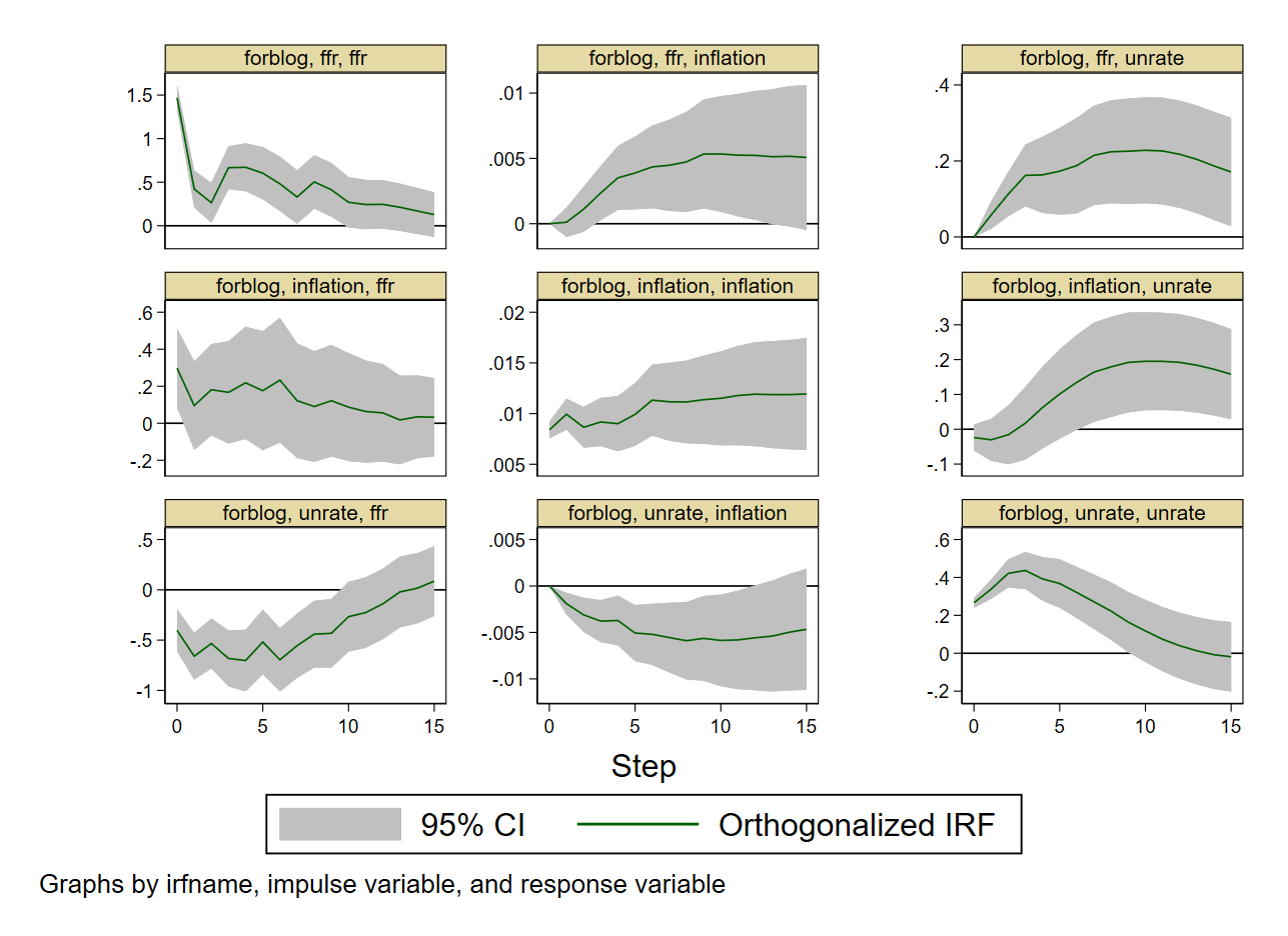
Figure 1: Graphs for Orthogonalized IRFs
Integrated Codes
 1
 2
 3
 4
 5
 6
 7
 8
 9
10
11
12
13
14
15
16
17
18
19
20
21
22
23
|
* load data
sysuse varsample.dta, clear

* set time series
tsset yq

* choose lag orders
varsoc inflation unrate ffr, maxlag(8)

* estimate VAR using `var' command
var inflation unrate ffr, lags(1/7)

* estimate VAR using `svar' command
matrix A1 = (1,0,0 \ .,1,0 \ .,.,1)
matrix B1 = (.,0,0 \ 0,.,0 \ 0,0,.)
svar inflation unrate ffr, lags(1/7) aeq(A1) beq(B1)

* crete output dataset myirf.irf
irf create forblog, step(15) set(myirf) replace

* visualize irfs
irf graph oirf, impulse(inflation unrate ffr) response(inflation unrate ffr) yline(0,lcolor(black)) xlabel(0(5)15) byopts(yrescale)
irf table oirf, impulse(inflation unrate ffr) response(inflation) noci
|
Summary
In this blog, I show how to use the integrated order var and svar to produce stylized outputs of VAR estimation in Stata. They will be benchmarks for the next blog where I will manually replicate all these results in Stata to obtain deeper understanding about these outputs.
References
- Vector autoregressions in Stata by David Schenck
- Stata handbook on svar command