Motivation
The motivation to clean this dataset is from Mukherjee et al. (2021, JFE). In this paper, the authors documented that one can get ahead-of-announcement estimation about the storage hubs for crude oil in the US from satellite images and trade on it. This will decrease the market reaction around the release of official figures because the oil storage information has been partially revealed during the traders’ arbitrage before announcement due to traders’ use of satellite images. To establish the causality between traders’ satellite image use and the lower market reaction around official figure release, this paper adopted cloudiness in the storage sites as Instrument Variable because the satellite images will be more obscure and thus less useful when the weather is cloudy. It turns out that the lowered market reaction is indeed less prominent during cloudy weeks.
In this article, I tried to construct a high-frequency cloudiness variable following the Mukherjee paper.
Data Source
The original data source is National Oceanic and Atmospheric Administration and I downloaded the Integrated Surface Database (ISD) dataset from its FTP server.
Brief Introduction to ISD dataset
The Integrated Surface Database (ISD) consists of global hourly and synoptic observations compiled from numerous sources into a single common ASCII format and common data model.
The database includes over 35,000 stations worldwide, with some having data as far back as 1901, though the data show a substantial increase in volume in the 1940s and again in the early 1970s. Currently, there are over 14,000 “active” stations updated daily in the database.
Station Number
Subsample Used In This Article
- Period: 2000 - 2020
- Station Range: 2168 Stations located in China (Range from 50136 to 59951)
- Freqency: Every 3 hours
Original Data Structure
-
The folders are named by year

Figure 1: NOAA Folder List -
For each year, there is individual file for each station
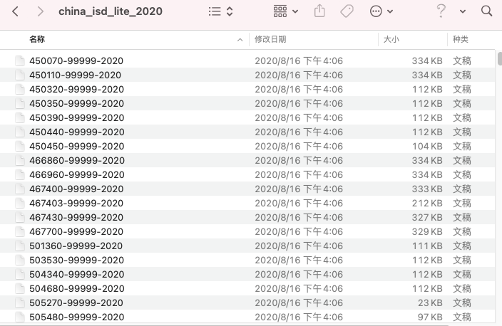
Figure 2: NOAA ISD File List -
For each file in a given year, the naming format is “Station ID-NCDC WBAN Number-Year”
-
For each file (with a relative station id and year), there are 12 columns

Figure 3: Sample ISD File -
Variable Definitions
Integrated Surface Data - Lite
Format Documentation
June 20, 2006
Introduction
The ISD-Lite data contain a fixed-width formatted subset of the complete Integrated Surface Data (ISD) for a select number of observational elements. The data are typically stored in a single file corresponding to the ISD data, i.e. one file per station per year. For more information on the ISD-Lite format, consult the ISD-Lite technical document.
Data Format
Field 1: Pos 1-4, Length 4: Observation Year
Year of observation, rounded to nearest whole hour
Field 2: Pos 6-7, Length 2: Observation Month
Month of observation, rounded to nearest whole hour
Field 3: Pos 9-11, Length 2: Observation Day
Day of observation, rounded to nearest whole hour
Field 4: Pos 12-13, Length 2: Observation Hour
Hour of observation, rounded to nearest whole hour
Field 5: Pos 14-19, Length 6: Air Temperature
The temperature of the air
UNITS: Degrees Celsius
SCALING FACTOR: 10
MISSING VALUE: -9999
Field 6: Pos 20-24, Length 6: Dew Point Temperature
The temperature to which a given parcel of air must be cooled at constant pressure and water vapor content in order for saturation to occur.
UNITS: Degrees Celsius
SCALING FACTOR: 10
MISSING VALUE: -9999
Field 7: Pos 26-31, Length 6: Sea Level Pressure
The air pressure relative to Mean Sea Level (MSL).
UNITS: Hectopascals
SCALING FACTOR: 10
MISSING VALUE: -9999
Field 8: Pos 32-37, Length 6: Wind Direction
The angle, measured in a clockwise direction, between true north and the direction from which the wind is blowing.
UNITS: Angular Degrees
SCALING FACTOR: 1
MISSING VALUE: -9999
*NOTE: Wind direction for calm winds is coded as 0.
Field 9: Pos 38-43, Length 6: Wind Speed Rate
The rate of horizontal travel of air past a fixed point.
UNITS: meters per second
SCALING FACTOR: 10
MISSING VALUE: -9999
Field 10: Pos 44-49, Length 6: Sky Condition Total Coverage Code
The code that denotes the fraction of the total celestial dome covered by clouds or other obscuring phenomena.
MISSING VALUE: -9999
DOMAIN:
0: None, SKC or CLR
1: One okta - 1/10 or less but not zero
2: Two oktas - 2/10 - 3/10, or FEW
3: Three oktas - 4/10
4: Four oktas - 5/10, or SCT
5: Five oktas - 6/10
6: Six oktas - 7/10 - 8/10
7: Seven oktas - 9/10 or more but not 10/10, or BKN
8: Eight oktas - 10/10, or OVC
9: Sky obscured, or cloud amount cannot be estimated
10: Partial obscuration
11: Thin scattered
12: Scattered
13: Dark scattered
14: Thin broken
15: Broken
16: Dark broken
17: Thin overcast
18: Overcast
19: Dark overcast
Field 11: Pos 50-55, Length 6: Liquid Precipitation Depth Dimension - One Hour Duration
The depth of liquid precipitation that is measured over a one hour accumulation period.
UNITS: millimeters
SCALING FACTOR: 10
MISSING VALUE: -9999
NOTE: Trace precipitation is coded as -1
Field 12: Pos 56-61, Length 6: Liquid Precipitation Depth Dimension - Six Hour Duration
The depth of liquid precipitation that is measured over a six hour accumulation period.
UNITS: millimeters
SCALING FACTOR: 10
MISSING VALUE: -9999
NOTE: Trace precipitation is coded as -1
Processing Data
Step 1: Extract Data From FTP Server
Suppose we already have a pre-specified station list and need to extract data files only for those stations from the FTP server.
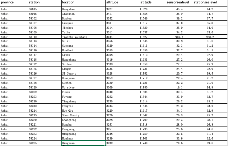
To complete this work, you need to
- Find out the file names in the FTP server for each station respectively
- For example, data in year 2019 for station 58015 has name
580150-99999-2019.gz - We could infer the names in FTP server contains three parts
- Station ID (5 digits) followed by a “0”
- NCDC WBAN Number (typically
99999for Chinese stations) - Record year
- For example, data in year 2019 for station 58015 has name
- Filter out the data files in the FTP server which belongs to the pre-specified station id list
- Copy the selected data files to your local folder
|
|
Step 2: Prepare Data
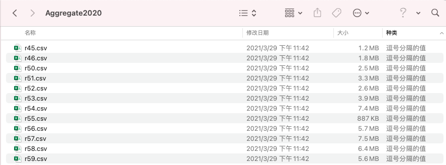
As the number of ISD files is too big, it will create too many redundent dta files when writing those datasets into Stata. Here I wrote all the ISD files recording data for the same first two-digit station ids in a same year into a new file, named by the first two-digit of station ids and store it into the folder “china_isd_lite_” + the respect year. This procedure is implemented in Python. All the following steps are implemented in Stata.
|
|
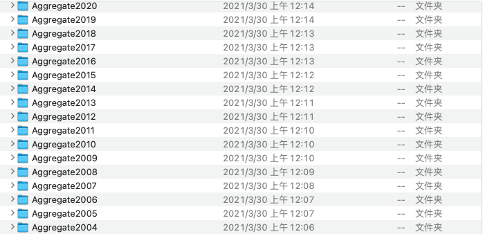
After this procedure, we should get folders for each year named by “Aggregate” + year.
In each folder, there should be a list of csv files named by the first two digits of station id.
Step 3: Write All ISD data in a Given Year Into A Same dta file
|
|
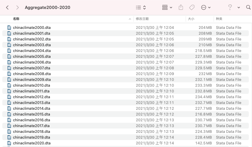
This step produces a series of dta files named as “chinaclimate” + year, which contains all isd data rows in a given year.
Step 4: Import Linktable in Order to Map Station Id into Province
The linktable is exactly the same as the station list we used in step 1. Suppose you name the imported linktable as linktable.dta
Step 5: Iterate Pre-cleaned Csv Files and Average Each Variable in Each Year
|
|
Step 6: Append All Province-Year Level Average Dta Files
|
|
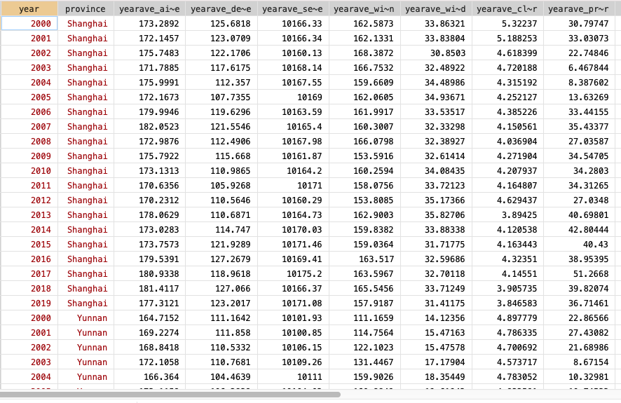
Sample Outcome
References
Mukherjee, Abhiroop, George Panayotov, and Janghoon Shon. 2021. “Eye in the Sky: Private Satellites and Government Macro Data.” Journal of Financial Economics, March. - PDF -
