Seeking Alpha From Market Participants' Information Acquisition Actions

Posted by Mengjie Xu on Thursday, September 8, 2022

Motivation

Just like the trading imbalance could be a powerful signal for upcoming stock price movement, investors’ information acquisition actions are also indicative for future security returns. According to Lee and So (2015), acquiring information is costly for investors and thus they only do so when the expected profits can cover the relative costs. Ceteris paribus, securities which attract more investor attention may have a higher likelihood of experiencing abnormal stock volatility from which a sophisticated investor can cultivate Alphas.

The information content of investors’ information acquisition actions has been well validated by a series of papers. For example, Da, Engelberg, and Gao (2011, JF) utilize search frequency in Google (Search Volume Index (SVI)) as a proxy for investor attention and show that firms with abnormally bigger Google search volume are more likely to have a higher stock price in the next 2 weeks and an eventual price reversal within the year, suggesting that the Google search volume may mainly capture the less sophisticated retail investors’ attention. Similarly, Drake, Johnson, Roulstone, and Thornock (2020, TAR) find that downloads number of a firm’s company filings filed in the EDGAR is significantly predictive of its subsequent performance and the predictive power is mainly driven by downloads from institutional investors’ IP address.

Employing news searching and news reading intensity for specific stocks on Bloomberg terminals as a new proxy for institutional investor attention, Ben-Rephael, Da, Israelsen (2017, RFS) and Easton, Ben-Repahael, Da, Israelsen (2021, TAR) more explicitly illustrated the lead-lag relationship between retail attention and institutional attention, suggesting that institutional investors are typically aware of the material firm-specific information earlier than retail investors and tend to make use of their information advantage by opportunistically providing liquidity when price pressure induced by retail investors arrives.

The take away from the literature is that by observing different market participants’ information acquisition actions in time-series, one can not only trace back how the current stock price was previously formulated, but also gain insights about how the stock price will evolve in the future.

The idea that predicting the stock movement from current market participants’ information acquisition actions, in my opinion, is especially fascinating: even though you have no idea about what exactly has happened to a specific firm, you could still get sense that there must be something abnormal when observing some unsual information acquisition actions targeted toward this firm in the market. From this perspective, approachable records of market participants’ information acquisition actions per se may facilitate the implicit dissemination of non-public material information in the market.

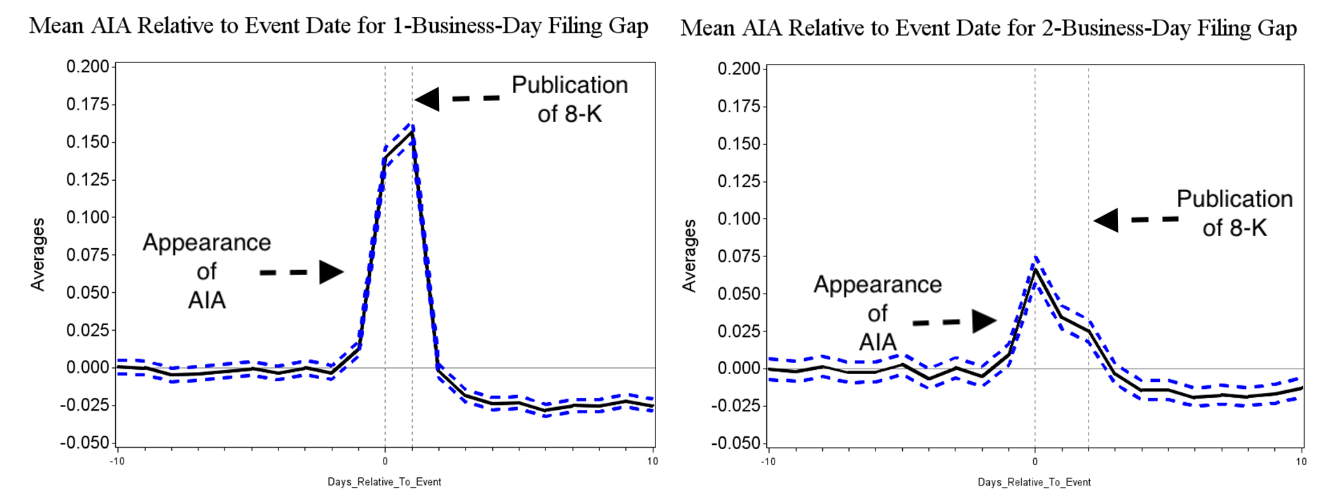
Take the stylized facts documented by Easton, Ben-Repahael, Da, Israelsen (2021, TAR) as an example. Figure 1 shows that when something material happens and a firm is obliged to file a 8-K to the SEC, one can always get informed days earlier than the publication of the 8-K filing by observing the abnormal Bloomberg Read Heat, depsite that he/she has no idea about what exactly has happened to the firm. Given the significant price pressure after the publication of 8-Ks, the information advantage means (potentially huge) trading profits.


Figure 1: Alphas From Abnormal Information Acquisition Actions

In this blog, I will introduce how to collect data and formulate the weekly measure for retail/institutional information acquisition actions. In particular, following Ben-Rephael, Da, Israelsen (2017, RFS) and Easton, Ben-Repahael, Da, Israelsen (2021, TAR), I will use Google Search Volume Index (SVI) to capture retail attention and Bloomberg institutional investors’ read heat to capture institutional information acquisition actions.

Formulate Retail Information Acquisition Measure (SVI)

As far as I know, the Google Search Volume Index (SVI) started to be recognized as a reasonable proxy for retail investors’ attention/information acquisition intensity in accounting and finance literature after the publication of Da, Engelberg, and Gao (2011, JF). The idea is that while institutional investors have more advanced platforms to gather information (e.g., Bloomberg, Reuters, etc), the majority of retail investors have to count on the Google search engine for information acquisition. Actually, the authors did find “a strong and direct link” between Google Search Volume Index (SVI) and retail order execution.

Following Da, Engelberg, and Gao (2011, JF), I will collect the weekly Google Search Volume Index (SVI) for each stock symbol, which could be then used for calculating the abnormal retail attention ASVI by substracting the rolling-average in the past 8 weeks from the current-week Google Search Volume Index (SVI).

Firstly, let’s randomly post two stock symbols and a date range and analyze how Google Trends API reacts to our post. Here I use tickers of Apple and Amazon, AAPL and AMZN, as search keywords. The date range is randomly specified as “2021-08-08 2022-08-08”.


Figure 2: Analysis Webpage

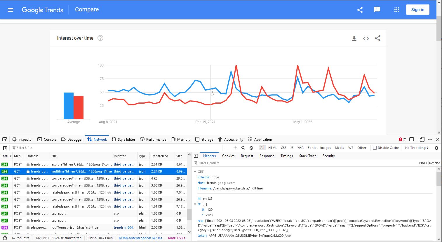
Figure 2 shows that the time series of the Search Volume Index is returned with json format and should contain ingredients when requesting as follows. In addition, one can also easily find out the cookies in the rendering results of the same reuqest.

Request method: GET

Base url: https://trends.google.com/trends/api/widgetdata/multiline

Request parameters:

 1
 2
 3
 4
 5
 6
 7
 8
 9
10
11
12
13
14
15
16
17
18
19
{
	"GET": {
		"scheme": "https",
		"host": "trends.google.com",
		"filename": "/trends/api/widgetdata/multiline",
		"query": {
			"hl": "en-US",
			"tz": [
				"-120",
				"-120"
			],
			"req": "{\"time\":\"2021-08-08 2022-08-08\",\"resolution\":\"WEEK\",\"locale\":\"en-US\",\"comparisonItem\":[{\"geo\":{},\"complexKeywordsRestriction\":{\"keyword\":[{\"type\":\"BROAD\",\"value\":\"aapl\"}]}},{\"geo\":{},\"complexKeywordsRestriction\":{\"keyword\":[{\"type\":\"BROAD\",\"value\":\"amzn\"}]}}],\"requestOptions\":{\"property\":\"\",\"backend\":\"IZG\",\"category\":0},\"userConfig\":{\"userType\":\"USER_TYPE_LEGIT_USER\"}}",
			"token": "APP6_UEAAAAAYxtcSHr7t2vjq6DYGSssMOgl0W-lpj05"
		},
		"remote": {
			"Address": "xxx.250.186.132:443"
		}
	}
}

By fetching the response message of the rendered url in the web browser, we can figure out the headers and the exact request url.

 1
 2
 3
 4
 5
 6
 7
 8
 9
10
11
12
13
14
await fetch("https://trends.google.com/trends/api/widgetdata/multiline?hl=en-US&tz=-120&req=%7B%22time%22:%222021-08-08+2022-08-08%22,%22resolution%22:%22WEEK%22,%22locale%22:%22en-US%22,%22comparisonItem%22:%5B%7B%22geo%22:%7B%7D,%22complexKeywordsRestriction%22:%7B%22keyword%22:%5B%7B%22type%22:%22BROAD%22,%22value%22:%22aapl%22%7D%5D%7D%7D,%7B%22geo%22:%7B%7D,%22complexKeywordsRestriction%22:%7B%22keyword%22:%5B%7B%22type%22:%22BROAD%22,%22value%22:%22amzn%22%7D%5D%7D%7D%5D,%22requestOptions%22:%7B%22property%22:%22%22,%22backend%22:%22IZG%22,%22category%22:0%7D,%22userConfig%22:%7B%22userType%22:%22USER_TYPE_LEGIT_USER%22%7D%7D&token=APP6_UEAAAAAYxtQ5U8DMlPHqyrSyWpmr2xkJaQQ-Ahb&tz=-120", {
    "credentials": "include",
    "headers": {
        "User-Agent": "Mozilla/5.0 (Windows NT 10.0; Win64; x64; rv:102.0) Gecko/20100101 Firefox/102.0",
        "Accept": "application/json, text/plain, */*",
        "Accept-Language": "en-US,en;q=0.5",
        "Sec-Fetch-Dest": "empty",
        "Sec-Fetch-Mode": "cors",
        "Sec-Fetch-Site": "same-origin"
    },
    "referrer": "https://trends.google.com/trends/explore?date=2021-08-08%202022-08-08&q=aapl,amzn",
    "method": "GET",
    "mode": "cors"
});

After the simple decoding of the request url, one can find out the request url is exactly the combination of the base url and specified parameters.

1
https://trends.google.com/trends/api/widgetdata/multiline?hl=en-US&tz=-120&req={"time":"2021-08-08+2022-08-08","resolution":"WEEK","locale":"en-US","comparisonItem":[{"geo":{},"complexKeywordsRestriction":{"keyword":[{"type":"BROAD","value":"aapl"}]}},{"geo":{},"complexKeywordsRestriction":{"keyword":[{"type":"BROAD","value":"amzn"}]}}],"requestOptions":{"property":"","backend":"IZG","category":0},"userConfig":{"userType":"USER_TYPE_LEGIT_USER"}}&token=APP6_UEAAAAAYxtQ5U8DMlPHqyrSyWpmr2xkJaQQ-Ahb&tz=-120

Analyze Parameter Structure

A typical set of post parameters is as follows.

1
2
3
4
5
6
hl: en-US
tz[...]
0:-120
1:-120
req:{"time":"2021-08-08 2022-08-08","resolution":"WEEK","locale":"en-US","comparisonItem":[{"geo":{},"complexKeywordsRestriction":{"keyword":[{"type":"BROAD","value":"aapl"}]}},{"geo":{},"complexKeywordsRestriction":{"keyword":[{"type":"BROAD","value":"amzn"}]}}],"requestOptions":{"property":"","backend":"IZG","category":0},"userConfig":{"userType":"USER_TYPE_LEGIT_USER"}}
token: APP6_UEAAAAAYxtQ5U8DMlPHqyrSyWpmr2xkJaQQ-Ahb

My little experiment shows that there are in general three components of the parameters.

  1. Relatively Fixed Part

    • The parameter hl specifies host language for accessing Google Trends, by default en-US
    • The parameter tz specifies time zone offset (in minutes). For example 360 means UTC -6 which is US CST
1
2
3
4
hl: en-US
tz[...]
0:-120
1:-120
  1. Variable Core Part

    • The parameter req consists of the following sub-parameters

      • time: time frame for search, in our sample case is 2021-08-08 2022-08-08

      • resolution: frequency of returned time series, in our sample case is WEEK, could also be HOUR, DAY or MONTH. There are different limitations for the span of the date range under different resolution levels.

      • locale: en-US, same as hl

      • comparisonItem: information about the search keywords, each keyword has a parallel complete post structure with following format

      1
      
          {"geo":{},"complexKeywordsRestriction":{"keyword":[{"type":"BROAD","value":"aapl"}]}}
      
      • requestOptions: typically fixed{"property":"","backend":"IZG","category":0}

      • userConfig: {"userType":"USER_TYPE_LEGIT_USER"}. Might be different if you post those parameters using algorithms. I will elaborate the details later.

    • The parameter token is the password for configuration from Google. This encrypted parameter needs another request. I will elaborate the details later.

      1
      
      token: APP6_UEAAAAAYxtQ5U8DMlPHqyrSyWpmr2xkJaQQ-Ahb
      

In sum, we can fill most parameters with the information we have in hand, such as the keyword list [‘AAPL’, ‘AMZN’] and the search range 2021-08-08 2022-08-08. The only obstacle left is that we have no idea how does Google encrypts those parameters and generate the dynamic secrets token.

Don’t worry. I will show how to get access to those encrypted tokens in the next subsection.
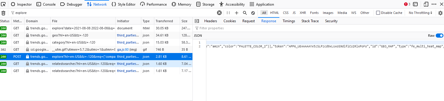
Find Out Tokens

With more checks on the page source, I find that the tokens are also returned with the format of json and can be accessed by posting the basic searching parameters to another url https://trends.google.com/trends/api/explore.


Figure 3: Find Out Tokens

With the similar procedures as those in the previous subsection. I find the parameter structure for this request is as follows.

 1
 2
 3
 4
 5
 6
 7
 8
 9
10
11
12
13
14
15
16
17
18
{
   "POST": {
   	"scheme": "https",
   	"host": "trends.google.com",
   	"filename": "/trends/api/explore",
   	"query": {
   		"hl": "en-US",
   		"tz": [
   			"-120",
   			"-120"
   		],
   		"req": "{\"comparisonItem\":[{\"keyword\":\"aapl\",\"geo\":\"\",\"time\":\"2021-08-08 2022-08-08\"},{\"keyword\":\"amzn\",\"geo\":\"\",\"time\":\"2021-08-08 2022-08-08\"}],\"category\":0,\"property\":\"\"}"
   	},
   	"remote": {
   		"Address": "142.250.186.132:443"
   	}
   }
}

Apparently, there is no information that is beyond our information set in this set of parameters.

The compressed returned json is as follows, from which one can easily find out the tokens and all the other parameters in need. Note that in addition to the time series of Google Search Index, this request also returns tokens for other type of information, such as data of geographical distributionGEO_MAP and keyword lists that are typically searched together with the focal keywordRELATED_QUERIES. Here I only display returned information, especially the token, for time series of Google Search Index.

Simply compare the following returned json in this subsection and the request parameters for the extracting of the time series data in the previous subsection, one will find that all the core variable parameters, req and token, needed in the previous subsection are contained in the following returned json.

 1
 2
 3
 4
 5
 6
 7
 8
 9
10
11
12
13
14
15
16
17
18
19
20
21
22
23
24
25
26
27
28
29
30
31
32
33
34
35
36
37
38
39
40
41
42
43
44
45
46
47
48
49
50
51
52
53
54
55
56
57
58
59
60
61
62
63
64
65
66
67
68
69
70
{
  "widgets":[
     {
        "request":{
           "time":"2021-08-08 2022-08-08",
           "resolution":"WEEK",
           "locale":"en-US",
           "comparisonItem":[
              {
                 "geo":{
                    
                 },
                 "complexKeywordsRestriction":{
                    "keyword":[
                       {
                          "type":"BROAD",
                          "value":"aapl"
                       }
                    ]
                 }
              },
              {
                 "geo":{
                    
                 },
                 "complexKeywordsRestriction":{
                    "keyword":[
                       {
                          "type":"BROAD",
                          "value":"amzn"
                       }
                    ]
                 }
              }
           ],
           "requestOptions":{
              "property":"",
              "backend":"IZG",
              "category":0
           },
           "userConfig":{
              "userType":"USER_TYPE_LEGIT_USER"
           }
        },
        "lineAnnotationText":"Search interest",
        "bullets":[
           {
              "text":"aapl"
           },
           {
              "text":"amzn"
           }
        ],
        "showLegend":false,
        "showAverages":true,
        "helpDialog":{
           "title":"Interest over time",
           "content":"Numbers represent search interest relative to the highest point on the chart for the given region and time. A value of 100 is the peak popularity for the term. A value of 50 means that the term is half as popular. A score of 0 means there was not enough data for this term."
        },
        "token":"APP6_UEAAAAAYxtcSHr7t2vjq6DYGSssMOgl0W-lpj05",
        "id":"TIMESERIES",
        "type":"fe_line_chart",
        "title":"Interest over time",
        "template":"fe",
        "embedTemplate":"fe_embed",
        "version":"1",
        "isLong":true,
        "isCurated":false
     }
     ]

Algorithm

For now, we have figured out all the necessary ingredients for writing the algorithm of automating the downloads of Google Search Volume Index (SVI).

Step 0: Define global variables that will be repeatedly used.

Step 1: Post the search keywords as well as the date range to https://trends.google.com/trends/api/explore and get the tokens as well as the parameters for the next step.

Step 2: Use the parameters obtained in Step 1 to obtain the time series Google Search Volume Index from https://trends.google.com/trends/api/widgetdata/multiline

Step 3: Clean the raw time series data and write it into the file.

Step 0: Define global variables

 1
 2
 3
 4
 5
 6
 7
 8
 9
10
11
12
13
14
15
16
17
18
19
20
21
22
23
24
25
26
class gtparas(object):
   tokenurl = "https://trends.google.com/trends/api/explore"
   tsurl = "https://trends.google.com/trends/api/widgetdata/multiline"
   headers = {
               "User-Agent": "Mozilla/5.0 (Windows NT 10.0; Win64; x64; rv:102.0) Gecko/20100101 Firefox/102.0",
               "Accept": "text/html,application/xhtml+xml,application/xml;q=0.9,image/avif,image/webp,*/*;q=0.8",
               "Accept-Language": "en-US,en;q=0.5",
               "Alt-Used": "trends.google.com",
               "Upgrade-Insecure-Requests": "1",
               "Sec-Fetch-Dest": "document",
               "Sec-Fetch-Mode": "navigate",
               "Sec-Fetch-Site": "none",
               "Sec-Fetch-User": "?1"
           }
   cookies = {
       "AEC": "AakniGMZ6nXlsuXNYf-cVEy-z26kpLEg-_E-OHRlDx-o4ApEe6xoCanQRw", 
       "CONSENT": "PENDING+772", 
       "SOCS": "CAISHAgBEhJnd3NfMjAyMjA4MzEtMF9SQzEaAmRlIAEaBgiA1c-YBg", 
       "NID": "511=BOJuzRwaQjxlv1xhQxBRom1aMkVL7CFU1RzfvcARIcHraZHPpuF_ZuCoFJ0YlmH18CbkapTUPEjBR6wm-U15jn_OT4yiyLy5WuMlBVvfSA7FNZ_tvrteTBgHRwXJcfJCC1VhZ0RbWlV881OpXOae007aMkwxgcjaGOZUEdQpd5NTV03c52iMD2jtVJUIyvsg6zU", 
       "__utmc": "10102256", 
       "__utmt": "1", 
       "__utma": "10102256.1871926219.1662307048.1662307048.1662307048.1", 
       "__utmb": "10102256.2.9.1662307053878", 
       "__utmz": "10102256.1662307048.1.1.utmcsr=(direct)|utmccn=(direct)|utmcmd=(none)"
       }
   

Step 1: Get Tokens

Input:

  • kw_list: keyword list, must be lower case, at maximum 5, e.g., ['appl', 'amzn']
  • daterange: search range, with format like 2021-08-08 2022-08-08
 1
 2
 3
 4
 5
 6
 7
 8
 9
10
11
12
13
14
15
16
def getoken(kw_list, daterange):
   token_payload = {
           'hl': "en-US",
           'tz': -120,
           'req': {'comparisonItem': [], 'category': 0, 'property': ''}
       }
   for kw in kw_list:
       keyword_payload = {'keyword': kw.lower(), 'geo': '',
                              'time': daterange}
       token_payload['req']['comparisonItem'].append(keyword_payload)
   token_payload['req'] = json.dumps(token_payload['req'])
   
   con = requests.post(gtparas.tokenurl, headers = gtparas.headers, cookies=gtparas.cookies, params = token_payload)
   widgets = json.loads(con.text[5:])['widgets']
   reqparas = recordtokens(widgets)
   return reqparas

In case one also want to obtain other type of information such as the geographical distribution of the Google search, I recorded all the returned tokens and parameters in this step.

 1
 2
 3
 4
 5
 6
 7
 8
 9
10
def recordtokens(widgets):
   reqparas = ""
   with open("toknes.txt", 'a') as f:
       for widget in widgets:
           if 'token' in widget.keys() and 'request' in widget.keys():
               del widget['helpDialog']
               f.write(str(widget)+",\n")
           if widget['id'] == 'TIMESERIES':
               reqparas = widget
   return reqparas

The output of this step reqparas contains necessary parameters request and token for the request of time series Search Volume Index.

1
{'request': {'time': '2017-08-06 2022-09-06', 'resolution': 'WEEK', 'locale': 'en-US', 'comparisonItem': [{'geo': {}, 'complexKeywordsRestriction': {'keyword': [{'type': 'BROAD', 'value': 'aapl'}]}}, {'geo': {}, 'complexKeywordsRestriction': {'keyword': [{'type': 'BROAD', 'value': 'amzn'}]}}], 'requestOptions': {'property': '', 'backend': 'IZG', 'category': 0}, 'userConfig': {'userType': 'USER_TYPE_SCRAPER'}}, 'lineAnnotationText': 'Search interest', 'bullets': [{'text': 'aapl'}, {'text': 'amzn'}], 'showLegend': False, 'showAverages': True, 'token': 'APP6_UEAAAAAYxsGftESZzXrrXfS82XnJlzqaOXskCAk', 'id': 'TIMESERIES', 'type': 'fe_line_chart', 'title': 'Interest over time', 'template': 'fe', 'embedTemplate': 'fe_embed', 'version': '1', 'isLong': True, 'isCurated': False}

Step 2: Request Time Series of Search Volume Index

The input keyword list and date range is exactly the same as in Step 1. Parameter req and token are both inherited from the output of the Step 1 reqparas.

 1
 2
 3
 4
 5
 6
 7
 8
 9
10
11
12
13
14
15
def fetchdata(kw_list, daterange):
    reqparas = getoken(kw_list, daterange)

    time.sleep(3)

    params = {
        "hl": "en-US",
        "tz": -120,
        "req" : json.dumps(reqparas['request']),
        "token": reqparas['token']
    }

    con = requests.get(gtparas.tsurl, headers=gtparas.headers, cookies=gtparas.cookies, params = params)
    req_json = json.loads(con.text[5:])
    return req_json

The output is json-formatted time series of Search Volume Index. The typical format is as following.

1
2
3
{"default":{"timelineData":[{"time":"1628380800","formattedTime":"Aug 8 \u2013 14, 2021","formattedAxisTime":"Aug 8, 2021","value":[54,34],"hasData":[true,true],"formattedValue":["54","34"]},{"time":"1628985600","formattedTime":"Aug 15 \u2013 21, 2021","formattedAxisTime":"Aug 15, 2021","value":[53,38],"hasData":[true,true],
...
,"formattedValue":["43","57"]},{"time":"1659830400","formattedTime":"Aug 7 \u2013 13, 2022","formattedAxisTime":"Aug 7, 2022","value":[44,48],"hasData":[true,true],"formattedValue":["44","48"]}],"averages":[50,43]}}

Step 3: Clean and Save Data

The input conatins

  • req_json: Json-formatted time series, output of Step 2
  • savefile: File to store the returned results, e.g., “GTRES_20220908.csv”
  • kw_list: List of search keywords. Properties are the same as in Step 1.
 1
 2
 3
 4
 5
 6
 7
 8
 9
10
11
12
13
14
15
16
def dealjson(req_json, savefile, kw_list):
    df = pd.DataFrame(req_json['default']['timelineData'])
    if (df.empty):
        return df

    df['date'] = pd.to_datetime(df['time'].astype(dtype='float64'),
                    unit='s')
    df = df.set_index(['date']).sort_index()
    result_df = df['value'].apply(lambda x: pd.Series(
        str(x).replace('[', '').replace(']', '').split(',')))
    for idx, kw in enumerate(kw_list):
        result_df.insert(len(result_df.columns), kw, result_df[idx].astype('int'))
        del result_df[idx]

    final = result_df.stack()
    final.to_csv(savefile, index=True, header=None, mode='a') 

The raw dataframe structure is as following.

time formattedTime formattedAxisTime value hasData formattedValue
1399161600 May 4 - 10, 2014 4-May-14 [96, 5, 0] [True, True, False] [‘96’, ‘5’, ‘0’]
1399766400 May 11 - 17, 2014 11-May-14 [80, 6, 4] [True, True, True] [‘80’, ‘6’, ‘4’]
1400371200 May 18 - 24, 2014 18-May-14 [97, 6, 3] [True, True, True] [‘97’, ‘6’, ‘3’]
1400976000 May 25 - 31, 2014 25-May-14 [86, 6, 5] [True, True, True] [‘86’, ‘6’, ‘5’]
1401580800 Jun 1 - 7, 2014 1-Jun-14 [82, 5, 3] [True, True, True] [‘82’, ‘5’, ‘3’]
1402185600 Jun 8 - 14, 2014 8-Jun-14 [76, 8, 5] [True, True, True] [‘76’, ‘8’, ‘5’]
1402790400 Jun 15 - 21, 2014 15-Jun-14 [87, 6, 2] [True, True, True] [‘87’, ‘6’, ‘2’]
1403395200 Jun 22 - 28, 2014 22-Jun-14 [74, 3, 2] [True, True, True] [‘74’, ‘3’, ‘2’]
1404000000 Jun 29 - Jul 5, 2014 29-Jun-14 [74, 0, 0] [True, False, False] [‘74’, ‘0’, ‘0’]
1404604800 Jul 6 - 12, 2014 6-Jul-14 [84, 3, 2] [True, True, True] [‘84’, ‘3’, ‘2’]
1405209600 Jul 13 - 19, 2014 13-Jul-14 [71, 5, 2] [True, True, True] [‘71’, ‘5’, ‘2’]

To make sure the columns are comparable among different requests, the formatted and saved dataframe structure has a panel-data format.

Date Symbol SVI
5/4/2014 DRIV 96
5/4/2014 DRNA 5
5/4/2014 DRQ 0
5/4/2014 DRRX 1
5/11/2014 DRII 5
5/11/2014 DRIV 80
5/11/2014 DRNA 6
5/11/2014 DRQ 4
5/11/2014 DRRX 2
5/18/2014 DRII 2
5/18/2014 DRIV 97
5/18/2014 DRNA 6
5/18/2014 DRQ 3
5/18/2014 DRRX 4
5/25/2014 DRII 0
5/25/2014 DRIV 86
5/25/2014 DRNA 6
5/25/2014 DRQ 5
5/25/2014 DRRX 2

Collect Raw SVI

  1
  2
  3
  4
  5
  6
  7
  8
  9
 10
 11
 12
 13
 14
 15
 16
 17
 18
 19
 20
 21
 22
 23
 24
 25
 26
 27
 28
 29
 30
 31
 32
 33
 34
 35
 36
 37
 38
 39
 40
 41
 42
 43
 44
 45
 46
 47
 48
 49
 50
 51
 52
 53
 54
 55
 56
 57
 58
 59
 60
 61
 62
 63
 64
 65
 66
 67
 68
 69
 70
 71
 72
 73
 74
 75
 76
 77
 78
 79
 80
 81
 82
 83
 84
 85
 86
 87
 88
 89
 90
 91
 92
 93
 94
 95
 96
 97
 98
 99
100
101
102
103
104
105
106
107
108
109
import requests  
import json
import pandas as pd
import urllib.parse
from datetime import datetime, timedelta
import os
from random import randint
import time
from math import floor
from tqdm import tqdm

class gtparas(object):

    tokenurl = "https://trends.google.com/trends/api/explore"
    tsurl = "https://trends.google.com/trends/api/widgetdata/multiline"

    headers = {
                "User-Agent": "Mozilla/5.0 (Windows NT 10.0; Win64; x64; rv:102.0) Gecko/20100101 Firefox/102.0",
                "Accept": "text/html,application/xhtml+xml,application/xml;q=0.9,image/avif,image/webp,*/*;q=0.8",
                "Accept-Language": "en-US,en;q=0.5",
                "Alt-Used": "trends.google.com",
                "Upgrade-Insecure-Requests": "1",
                "Sec-Fetch-Dest": "document",
                "Sec-Fetch-Mode": "navigate",
                "Sec-Fetch-Site": "none",
                "Sec-Fetch-User": "?1"
            }

    cookies = {
        "AEC": "AakniGMZ6nXlsuXNYf-cVEy-z26kpLEg-_E-OHRlDx-o4ApEe6xoCanQRw", 
        "CONSENT": "PENDING+772", 
        "SOCS": "CAISHAgBEhJnd3NfMjAyMjA4MzEtMF9SQzEaAmRlIAEaBgiA1c-YBg", 
        "NID": "511=BOJuzRwaQjxlv1xhQxBRom1aMkVL7CFU1RzfvcARIcHraZHPpuF_ZuCoFJ0YlmH18CbkapTUPEjBR6wm-U15jn_OT4yiyLy5WuMlBVvfSA7FNZ_tvrteTBgHRwXJcfJCC1VhZ0RbWlV881OpXOae007aMkwxgcjaGOZUEdQpd5NTV03c52iMD2jtVJUIyvsg6zU", 
        "__utmc": "10102256", 
        "__utmt": "1", 
        "__utma": "10102256.1871926219.1662307048.1662307048.1662307048.1", 
        "__utmb": "10102256.2.9.1662307053878", 
        "__utmz": "10102256.1662307048.1.1.utmcsr=(direct)|utmccn=(direct)|utmcmd=(none)"
        }
    

def recordtokens(widgets):
    reqparas = ""
    with open("toknes.txt", 'a') as f:
        for widget in widgets:
            if 'token' in widget.keys() and 'request' in widget.keys():
                del widget['helpDialog']
                f.write(str(widget)+",\n")
            if widget['id'] == 'TIMESERIES':
                reqparas = widget
    return reqparas

def getoken(kw_list, daterange):
    token_payload = {
            'hl': "en-US",
            'tz': -120,
            'req': {'comparisonItem': [], 'category': 0, 'property': ''}
        }
    for kw in kw_list:
        keyword_payload = {'keyword': kw.lower(), 'geo': '',
                               'time': daterange}
        token_payload['req']['comparisonItem'].append(keyword_payload)
    token_payload['req'] = json.dumps(token_payload['req'])
    
    con = requests.post(gtparas.tokenurl, headers = gtparas.headers, cookies=gtparas.cookies, params = token_payload)
    widgets = json.loads(con.text[5:])['widgets']
    reqparas = recordtokens(widgets)
    return reqparas

def dealjson(req_json, savefile, kw_list):
    df = pd.DataFrame(req_json['default']['timelineData'])

    df.to_csv("test1.csv")
    if (df.empty):
        return df

    df['date'] = pd.to_datetime(df['time'].astype(dtype='float64'),
                    unit='s')
    df = df.set_index(['date']).sort_index()
    result_df = df['value'].apply(lambda x: pd.Series(
        str(x).replace('[', '').replace(']', '').split(',')))
    for idx, kw in enumerate(kw_list):
        result_df.insert(len(result_df.columns), kw, result_df[idx].astype('int'))
        del result_df[idx]

    final = result_df.stack()
    print(final)
    final.to_csv(savefile, index=True, header=None, mode='a') 

def fetchdata(kw_list, daterange):
    reqparas = getoken(kw_list, daterange)

    time.sleep(3)

    params = {
        "hl": "en-US",
        "tz": -120,
        "req" : json.dumps(reqparas['request']),
        "token": reqparas['token']
    }

    con = requests.get(gtparas.tsurl, headers=gtparas.headers, cookies=gtparas.cookies, params = params)
    req_json = json.loads(con.text[5:])
    dealjson(req_json, savefile, kw_list)
    
if __name__ == '__main__':
    kw_list = ['AAPL', 'AMZN', 'TSLA']
    daterange = '2021-08-08 2022-08-08'
    fetchdata(kw_list, daterange)

Formulate Institutional Information Acquisition Measure (AIA)

Bloomberg as the Data Source

To my knowledge, Ben-Rephael, Da, Israelsen (2017, RFS) was the first to use the Bloomberg Read Heat (AIA) was firstly as a proxy for institutional attention. According to their paper, Bloomberg records the number of times news articles on a particular stock are read by its terminal users and the number of times users actively search for news about a specific stock. … They assign a score of 0 if the rolling average is in the lowest 80% of the hourly counts over the previous 30 days. Similarly, Bloomberg assigns a score of 1, 2, 3 or 4 if the average is between 80% and 90%, 90% and 94%, 94% and 96%, or greater than 96% of the previous 30 days’ hourly counts, respectively. … Bloomberg aggregates up to the daily frequency by taking a maximum of all hourly scores throughout the calendar day.

Collect Bloomberg News Read Heat

In my previously blog Extract Mass Data Via Bloomberg API, I have displayed how to obtain a specific variable from Bloomberg via Bloomberg API. In this case, the variable of interest NEWS_HEAT_READ_DMAX. Maybe you also want to obtain some related variables like the number of news per day and the tone of the news, etc.

Then just request them from the Bloomberg.

 1
 2
 3
 4
 5
 6
 7
 8
 9
10
11
12
13
14
15
16
17
18
19
20
21
22
23
24
25
26
27
28
29
30
31
32
33
34
35
36
37
38
39
40
41
42
43
44
45
46
47
48
49
50
51
52
import pandas as pd
from xbbg import blp
from tqdm import tqdm
import csv

df = pd.read_excel('cusiplist.xlsx')

date_from = '20090101'
date_until = '20210630'
target = ['NEWS_HEAT_READ_DMAX', 'NEWS_HEAT_READ_DAVG','NEWS_HEAT_PUB_DAVG','NEWS_SENTIMENT_DAILY_AVG','NEWS_HEAT_PUB_DNUMSTORIES','NEWS_HEAT_PUB_DMAX','NEWS_NEG_SENTIMENT_COUNT','NEWS_POS_SENTIMENT_COUNT','NEWS_PUBLICATION_COUNT']

def prepare(temp):
    cols = [i[1] for i in temp.columns]
    diff = set(target) - set(cols)
    diffindex = [target.index(i) for i in diff]
    leftindex = set(range(len(target))) - set(diffindex)
    dictt = list(zip(range(len(cols)), leftindex))
    return([cols, dictt])

# Iterate each cusip in the cusip list
for i in tqdm(df.iterrows()):
  	# Obtain cusip
    cusip = i[1][2]
    # Request data from Bloomberg API
    temp = blp.bdh(tickers=cusip,flds=target, start_date=date_from,\
                   end_date=date_until, Per = 'Y')
    [cols, dictt] = prepare(temp)

    with open('Esg_Score_Multiple','a') as f:
      	# Open a csv file with mode 'a', which allows adding new rows
        # without covering existed rows
        g = csv.writer(f)
        # Create a list with length equal to the number of requested 
        # variables plus 3
        headline =['DATE']+target+['CUSIP', 'FIELDS']
        res = [""]*(len(target)+3)
        
        # Iterate each row of returned dataframe
        for row in temp.iterrows():
            for j,k  in dictt:
              	# Put date to the first cell
                res[0] = row[0]
                # Put variables returned by API following the
                # pre-specified order
                res[k+1] = row[1][j]
                # Put the identifier of security into the list
                res[len(target)+1] = cusip
                # Put names of valid variables returned for the security
                # into the last cell of the list for cross-check
                res[len(target)+2] = cols
            # Write the revised list to the opened csv file
            g.writerow(res)

Summary

In this blog, I showed the value of investors’ attention (or information acquisition actions) and introduced how to collect data for the purpose of formulating the proxies of retail attention and institutional attention respectively. Following Ben-Rephael, Da, Israelsen (2017, RFS) and Ben-Repahael, Da, Israelsen (2021, TAR) , I use Google Search Volume Index (SVI) to capture retail attention and news reading intensity for specific stocks on Bloomberg terminals as a new proxy for institutional investor attention.

References

Ben-Rephael, Azi, Zhi Da, and Ryan D. Israelsen. “It depends on where you search: Institutional investor attention and underreaction to news.” The Review of Financial Studies 30, no. 9 (2017): 3009-3047.

Da, Zhi, Joseph Engelberg, and Pengjie Gao. “In search of attention.” The Journal of Finance 66, no. 5 (2011): 1461-1499.

Drake, Michael S., Bret A. Johnson, Darren T. Roulstone, and Jacob R. Thornock. “Is there information content in information acquisition?.” The Accounting Review 95, no. 2 (2020): 113-139.

Lee, Charles MC, and Eric C. So. “Alphanomics: The informational underpinnings of market efficiency.” Foundations and Trends® in Accounting 9.2–3 (2015): 59-258.

Peter Easton, Azi Ben-Repahael, Zhi Da, Ryan Israelsen. “Who Pays Attention to SEC Form 8-K?.” The Accounting Review (2021)